Load an SFT from file
[1]:
import soapcw
import matplotlib.pyplot as plt
import numpy as np
Load an SFT from a file
[2]:
# load sft file between 100.5,100.6 Hz
sft = soapcw.cw.LoadSFT("./data/H10124_H1_1800SFT-F100.0_102.1.sft",fmin=100.5,fmax=100.6)
# normalise the SFT to its running median
sft.norm_rngmed()
# if there are gaps in the data, fill these with a constant value
sft.fill_gaps()
# sum the sfts over a day (default) or specify
sft.sum_sfts()
[4]:
# or for single line run
sft = soapcw.cw.LoadSFT("./data/H10124_H1_1800SFT-F100.0_102.1.sft",fmin=100.5,fmax=100.6,norm=True,summed=True,filled=True)
[3]:
# plot the spectrogram
fig, ax = plt.subplots(figsize=(15,8))
ax.imshow(sft.H1.summed_norm_sft_power.T,origin="lower",aspect="auto",cmap=plt.get_cmap("YlGnBu"))
[3]:
<matplotlib.image.AxesImage at 0x7fd35cfa3070>

Veto frequency bands from sft when loading
[6]:
vetolist = [100.55]
[7]:
sft_veto = soapcw.cw.LoadSFT("./data/H10124_H1_1800SFT-F100.0_102.1.sft",fmin=100.5,fmax=100.6,norm=True,summed=True,filled=True,vetolist = vetolist)
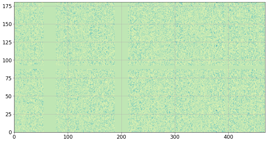
[8]:
# plot the spectrogram
fig, ax = plt.subplots(figsize=(15,8))
ax.imshow(sft_veto.H1.summed_norm_sft_power.T,origin="lower",aspect="auto",cmap=plt.get_cmap("YlGnBu"))
[8]:
<matplotlib.image.AxesImage at 0x10df2df50>
[ ]: